0.008mm accuracy with the OpenScan Mini - Tutorial - Mesh analysis using CloudCompare

TLDR:

I scanned a feeler gauge with the OpenScan Mini, processed the data in the OpenScan Cloud and scaled the object with the help of the known dimension. Next, I digitally measured the thickness of each feeler and got a deviation of 0.008 mm from the claimed/real thicknesses (0.05 mm - 0.55 mm). There are several points that will be discussed in this article. But just to give you a perspective, that 0.008 mm is somewhat around a fifth of the thickness of the human hair.

Since the beginning of the OpenScan project, the question of how accurate the device can be had been haunting. I have been very hesitant to even try to answer this question, since I am no metrology expert and my methods might be a bit funky. But I finally convinced myself, that the following measurements and discussion seem at least worth sharing. And hopefully, this could even start a discussion with some more experienced users. Maybe even some other scanner users or developers could do a similar scan with their devices and share the (raw) results. I would even do the analysis :)

I will use this case to show my standard procedure of analyzing the mesh in CloudCompare (which are both free-to-use programs).

The scan object and procedure: Feeler gauge

Source: https://www.amazon.de/-/en/3083-Precision-Feeler-Sheets-Metric/dp/B001ILD9HQ/ref=sxin_14_b2b_sx_ibs_v4_desktop

The feeler gauge is normally used to measure gap widths. I got mine for around 10€ and this should be at least an indicator for the quality and accuracy. The feeler's thickness range from 0.05 mm to 1 mm in steps of 0.05 mm. But I only used those in the range of 0.05-0.55 mm plus the 1 mm piece.

This is probably the ugliest scan object arrangement I ever did, but it is highly functional:

• I used some putty to give the object some depth, because the alignment of front and back seemed to be tricky/fail otherwise in earlier attempts
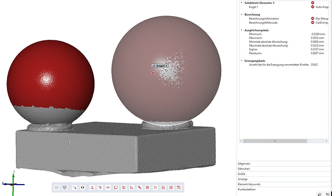
• added the gauge block of known dimensions. The width along the blue line (see below) is 50.000(5) mm and accurate to 0.5 microns according to DIN EN ISO 3650
• sprayed the whole arrangement with a light sprinkle of Aesub Orange to create enough surface features
• used the polarizer module of the OpenScan Mini to filter reflective highlights
• took a total of 150 photos with the Arducam IMX519

Raw scan result using the OpenScan Cloud, see and download the 3d model on Sketchfab

Cross-section along the red line (0.005 to 0.055 mm thickness)

Some observations:

• the noise in the bottom area of the scan is caused by the photos being mostly blurry in that area (since the object exceeds the 8x8x8cm scanning volume of the OpenScan Mini)
• in the area of interest (the feeler tips and the gauge block) have very low noise
• you can even see my fingerprints in the putty ;)

Scaling was done in Autodesk Meshmixer and the procedure will be covered in an upcoming tutorial. But basically I took three measurements along the blue line and scaled the object accordingly.

Analysis in CloudCompare

 Feel free to skip this chapter by jumping to the results ;)

 (1) Drag and Drop the .stl/.obj file into CloudCompare

If the object appears fully white, you should activate "Display --> Shaders & Filters --> EDL shader"

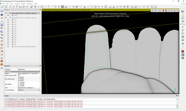
(2) Segment the object into smaller pieces

• Zoom into the area of interest and use "Edit --> Segment".
• Click into the 3d view to create a contour (green lines).
• Press "I" or "O" to keep the inner/outer segment. (Don't worry, the other part will be kept as well). This will create two new objects to work with.

(3) Rename the created objects and save everything

• Use the DB Tree window on the left to manage the individual parts. I like to rename each segment to keep it somewhat organized.
• Note, that CloudCompare has no undo-operation (!!) and thus you should save your progress from time to time.
• Therefore, select all objects in the DB Tree and "File --> Save". This will create .bin file, which you can reload at any time.

 (4) Sample Points (Mesh --> PointCloud)

• Hide all unneeded object by unticking the boxes in the DB Tree window.
• Select one of the segments (in my case, the "100" mesh, which is the left most feeler with a thickness of 1.00mm).
• Convert the Mesh to a point cloud with 1 Mio. Points with "Edit --> Mesh --> Sample Points"
• And hide the 100 mesh (since a 100.sampled object appears, which contains the samples point cloud)

(5) Segment into the upper and lower part

• Select the point cloud in the DB Tree (100.sampled)
• Use "Edit --> Segment" Tool and create a contour around the upper or lower part
• two point clouds 100.sampled.remaining and 100.sampled.segmented will be created

(6) Calculate the mean distance between the two objects

• "Tools --> Distances --> Cloud/Cloud Dist."
• Choose the role, when you are using for instance a CAD model as reference (doesn't matter here)
• Ok --> Compute --> Ok to create a colorful histogram ;)

(7) Showing the results (pt. 1)

• Select each point cloud in the DB Tree and deactivate the "Normals" in the Properties window (left side)
• Now, one of the point clouds appears in wonderful colors
• Note, that the mean distance and std. deviation between the two entities is displayed on the bottom of the main window (MEAN = 1.007713 and STD = 0.007364)

(8) Showing the results (pt. 2)

• Select the colored point cloud in the DB Tree
• "Edit --> Scalar fields --> Show Histogram"
• A new window will appear showing the histogram
• You can export the histogram as .png or the raw values as .csv on the top right of the window.

(9) Repeat for the other 11 feelers ;)

(Note, that I changed the scalar-field's x-axis a bit to get comparable color-coding. This doesn't have any influence on the mean and STD values shown below. If anyone is interested in the raw data, feel free to reach out ;)

I am really not sure, what to think about these results, so let's continue with some discussion:

Results and Discussion

Δd = 0,0077±0,0059 mm

(the mean difference between digitally measured and real/claimed thickness is roughly 0.007 micron)

Some thoughts and partly open questions:

What are the real dimensions of the individual feelers?

This is hard to tell, but I would say, that due to the low variance, they seemed to be surprisingly accurate.

How accurate and reliable is the scaling?

I repeated this scan and scanned some other objects too and seem to get consistent results.

What is the influence of the scanning spray?

As far as I know, the thickness of carefully applied Aesub Orange lies within the low single digit micron range (but maybe someone can verify/correct)

Did I do any other methodical mistakes??

I do not know, please point me into the right direction and share your thoughts!

Can I claim, that the OpenScan Mini can be accurate to 0.008mm (or 0.02mm to be a bit more conservative)??

I am still hesitant to claim this or any accuracy and would love to hear some professional opinions on that!

Thanks for your interest!

Best regards,

Thomas

PS: If you made it that far and like what I do, feel free to support the project through Patreon.